Module 1.4
Intro to the Tidyverse
- Make sure that the Tidyverse is installed. You can do this by running the
install.packages("tidyverse")command in the console if you have not done so already. - Familiarize yourself with the Tidyverse group of packages.
- We will not be using all of these, but the first four (
ggplot2,dplyr,tidyr, andreadr) are essential for this course. - Create and save a QMD file for this module in your Module 1 project folder.
Overview
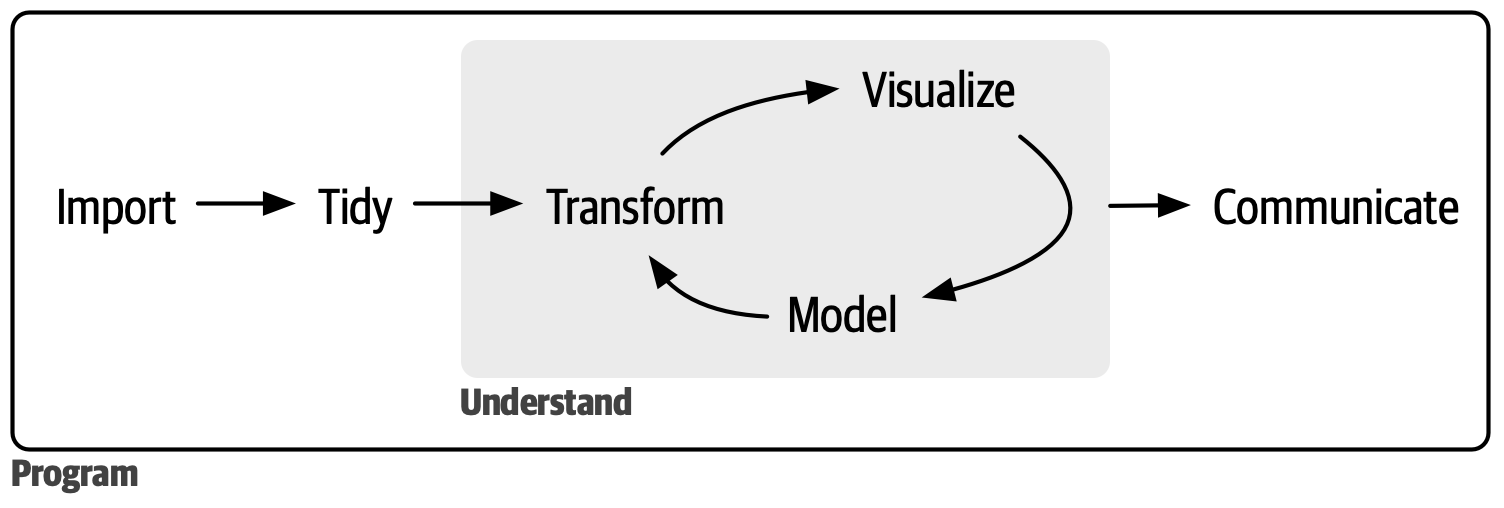
Data science involves a systematic workflow that takes us from raw data to meaningful insights. This journey typically includes data import, tidying, transformation, visualization, modeling, and communication of results. This is the workflow that we are going to be discussing for the rest of the course.
At the heart of this workflow and modern data science in R lies the Tidyverse, an ecosystem of packages designed to work harmoniously together. The Tidyverse represents not just a collection of tools but also a philosophy about how data analysis should be approached—with consistency, clarity, and a focus on human readability. To get a better sense of what the it is all about, watch this video of Hadley Wickham, the creator of the Tidyverse, discussing the importance of code maintenance and the evolution of the Tidyverse.
In this module, you’ll begin your journey with several core Tidyverse packages that form the foundation of data science work. While we will touch on most of the Tidyverse packages in this, course, there are four that are essential for our work:
-
readrstreamlines the process of importing data into R -
dplyrprovides intuitive verbs for data manipulation and transformation -
ggplot2enables creation of beautiful visualizations using the grammar of graphics -
tidyrwill be helpful when we want to reshape (pivot) our data Today, we are going to get a general sense of the Tidyverse. We will also talk about how to use thereadrpackage to read data into R and a couple of ways to view the contents of the data frame. Then we will coverggplot2in the next couple of modules anddplyrandtidyrwill come into focus next week when we turn to data wrangling.
Working with Tidyverse Packages
When using Tidyverse packages, you have a few options for how to load and access their functions.
Initially, we’ll load individual packages as needed. This approach helps you understand which functions come from which packages and allows you to be selective about which parts of the Tidyverse you’re using.
For example, to load the ggplot2 package you would go:
As you become more comfortable with the Tidyverse ecosystem, you might prefer to load all the core packages at once:
This command loads all of the core Tidyverse packages, including readr, ggplot2, dplyr, tidyr, and others.
Sometimes you might see code where the author loads a package using its namespace by using the :: operator, like this:
This will not be as common a workflow for us, but it is helpful in context where you want to use a function from a package without loading the entire package. This can be helpful when putting code into production or writing packages because it helps to avoid conflicts between functions and minimize resources.
Reading Data into R
The first step in most data analysis projects is importing your data. The readr package makes this process straightforward and efficient, especially when working with CSV files, which are one of the most common data formats.
Let’s start by loading the readr package and importing a dataset about democracy measures around the world. Download this data set and move it in your project folder as dem_summary.csv:
A best practice is to save your data files in a subfolder within your project directory. Usually we would call that folder “data” and reference the file as data/name_of_file.csv. This keeps your workspace organized and makes it easier to find your data files later.
Now try reading in the data and storing it in an object using the read_csv() function from the readr package like this:
When you run this code, readr will display a message showing how it interpreted each column (e.g., as character, numeric, etc.). This is helpful for quickly identifying if any columns were parsed incorrectly.
We could also have used the base R read function read.csv() to read in the data, but read_csv() is generally faster and more efficient. It also has a number of advantages over the base R function. For example, it automatically handles column types, so you don’t have to specify them manually. read_csv() also provides better handling of missing values and other common issues that can arise when importing data.
Viewing the Data
Once you’ve imported your data, it’s important to take a look at it to ensure everything looks correct. One way to do this is to type View() in your console or (equivalently) click on the name of the object in your Environment tab to see the data in a spreadsheet:
This will open a new tab in RStudio with a spreadsheet-like view of your data frame. This is a great way to get a quick overview of your data.
The glimpse() function from the dplyr package is another great way to get an overview of your data frame. It provides a quick summary of the data, including the number of rows and columns, the names of the columns, and the data types of each column.
Rows: 6
Columns: 5
$ region    <chr> "The West", "Latin America", "Eastern Europe", "Asia", "Afri…
$ polyarchy <dbl> 0.8709230, 0.6371358, 0.5387451, 0.4076602, 0.3934166, 0.245…
$ gdp_pc    <dbl> 37.913054, 9.610284, 12.176554, 9.746391, 4.410484, 21.134319
$ flfp      <dbl> 52.99082, 48.12645, 50.45894, 50.32171, 56.69530, 26.57872
$ women_rep <dbl> 28.12921, 21.32548, 17.99728, 14.45225, 17.44296, 10.21568
Here we see that the data frame consists of five columns: region; polyarchy (a measure of democracy); GDP per capita (gdp_pc); female labor force participation rates (flfp); and levels of women’s representation (women_rep). We also see that region is a character variable and the other four columns are numeric variables. Finally, we see that there are six rows in the data frame representing the average values of these variables for each region in the world.
Note that there are some other base R functions that can be useful for viewing data frames. You can use the head() function to view the first few rows of a data frame:
head(dem_summary)# A tibble: 6 × 5
region polyarchy gdp_pc flfp women_rep
<chr> <dbl> <dbl> <dbl> <dbl>
1 The West 0.871 37.9 53.0 28.1
2 Latin America 0.637 9.61 48.1 21.3
3 Eastern Europe 0.539 12.2 50.5 18.0
4 Asia 0.408 9.75 50.3 14.5
5 Africa 0.393 4.41 56.7 17.4
6 Middle East 0.246 21.1 26.6 10.2You can also use the tail() function to view the last few rows of a data frame:
tail(dem_summary)# A tibble: 6 × 5
region polyarchy gdp_pc flfp women_rep
<chr> <dbl> <dbl> <dbl> <dbl>
1 The West 0.871 37.9 53.0 28.1
2 Latin America 0.637 9.61 48.1 21.3
3 Eastern Europe 0.539 12.2 50.5 18.0
4 Asia 0.408 9.75 50.3 14.5
5 Africa 0.393 4.41 56.7 17.4
6 Middle East 0.246 21.1 26.6 10.2And the summary() function to get a summary of the data frame, including the minimum, maximum, mean, and median values for each column:
summary(dem_summary) region polyarchy gdp_pc flfp
Length:6 Min. :0.2459 Min. : 4.410 Min. :26.58
Class :character 1st Qu.:0.3970 1st Qu.: 9.644 1st Qu.:48.68
Mode :character Median :0.4732 Median :10.961 Median :50.39
Mean :0.5156 Mean :15.832 Mean :47.53
3rd Qu.:0.6125 3rd Qu.:18.895 3rd Qu.:52.36
Max. :0.8709 Max. :37.913 Max. :56.70
women_rep
Min. :10.22
1st Qu.:15.20
Median :17.72
Mean :18.26
3rd Qu.:20.49
Max. :28.13