Click on Code toggle below to unfold the setup code chunk. Then, copy and run the code in your Quarto notebook to load the necessary packages and create the data frame for this lesson.
In our last module, we explored tools available for examining categorical data—variables that capture groupings or labels, like regime type or world region. We looked at bar charts and how grouping by a categorical variable can help us uncover patterns in data. In this module, we turn our attention to continuous data.
Continuous variables are numeric measurements that can take on an infinite range of values within a given interval. Think of indicators like GDP per capita, population size, or life expectancy—these are variables that allow us to compare magnitude, observe variation, and investigate relationships between quantities.
In this lesson, we will learn how to explore continuous variables. We will look at different types of distributions and learn how to visualize a single continuous variable with histograms and density plots. Then we will look at how to compare distributions across groups using ridge plots.
What Does the Distribution Look Like?
To understand continuous variables, we often begin by examining their distribution through a visual representation of how values are spread out across the range with a histogram or a density plot. These shapes tell us a lot about the nature of the data and can guide our decisions about how to summarize or transform variables.
Let’s look at some histograms displaying common types of distributions you’re likely to encounter. A histogram shows how many observations fall into different ranges of values, allowing us to see patterns like skewness, modality, and clustering. They do this by grouping values into bins and counting how many observations fall into each one. Think of it as slicing up the number line into segments and stacking up bars based on how many countries fall into each slice.
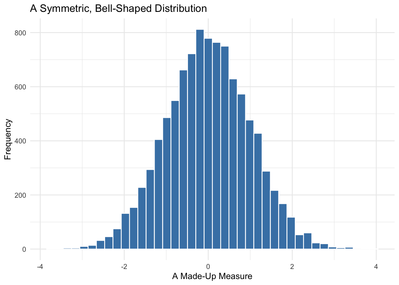
Symmetric and Bell-Shaped
When most values are clustered around the center, with fewer values tapering off evenly on both sides, we call the distribution symmetric or bell-shaped. This kind of distribution is common in physical measurements and standardized test scores. It’s also the foundation of many statistical techniques that assume normality.
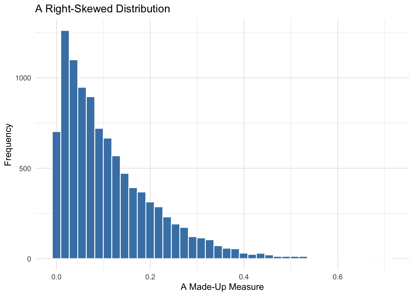
Right-Skewed
A right-skewed distribution (also known as positively skewed) has a long tail stretching to the right. This often occurs when values are bounded at zero but can stretch very far in the positive direction. GDP per capita is a classic example: most countries are clustered at the lower end, with a few very wealthy outliers pulling the tail to the right.
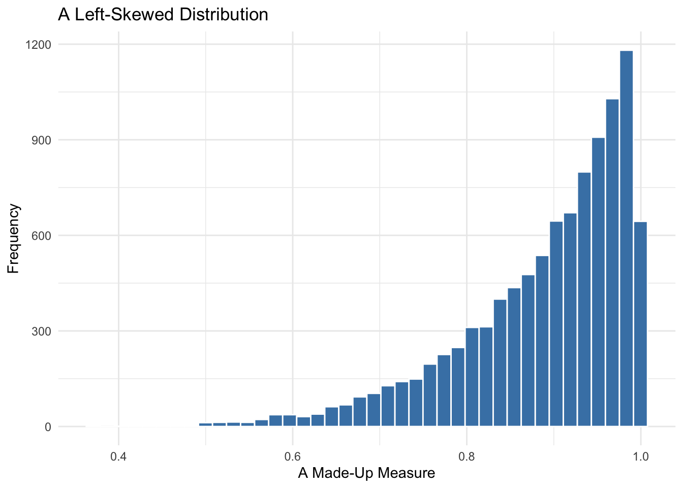
Left-Skewed
Less common, but still important, are left-skewed (negatively skewed) distributions, where the tail stretches to the left. This might happen with variables that have an upper bound, like survey responses with a maximum score, where a majority of responses are at the top end but a few fall below.
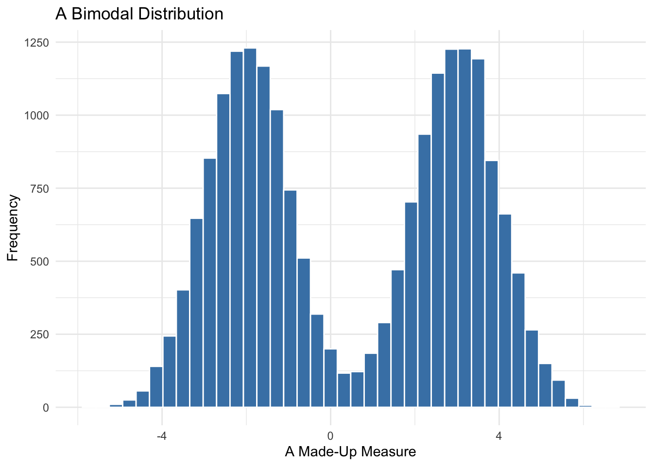
Bimodal
A bimodal distribution has two peaks — two distinct groups of values. This often signals that your data may actually come from two different populations. For example, if you combine data on voter turnout from democratic and authoritarian regimes, you might see one peak for each group.
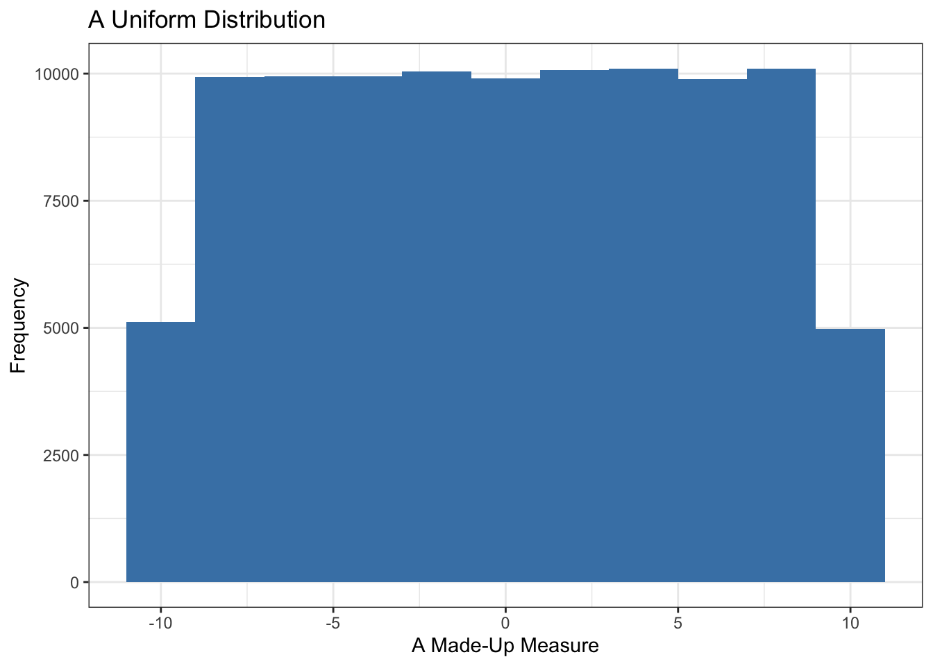
Uniform
A uniform distribution has no peaks or valleys — all values are equally likely. This is relatively rare in real-world data but can occur in random sampling or when measuring something that has been evenly distributed across a range.
Each of these shapes tells a different story about how values are distributed — and that story helps us decide how to summarize the variable. For example, when a distribution is symmetric, the mean and median are usually close together. But in a skewed distribution, the mean gets pulled toward the long tail, making it a less reliable summary on its own.
Creating a Histogram
Now that we have been exposed to a number of different types of distributions, lets practice making histograms so that we can explore continous data on our own. To make a histogram in ggplot2, we use the geom_histogram() function. This function takes an aesthetic mapping (aes()) that specifies which variable to plot on the x-axis, and it automatically counts how many observations fall into each bin.
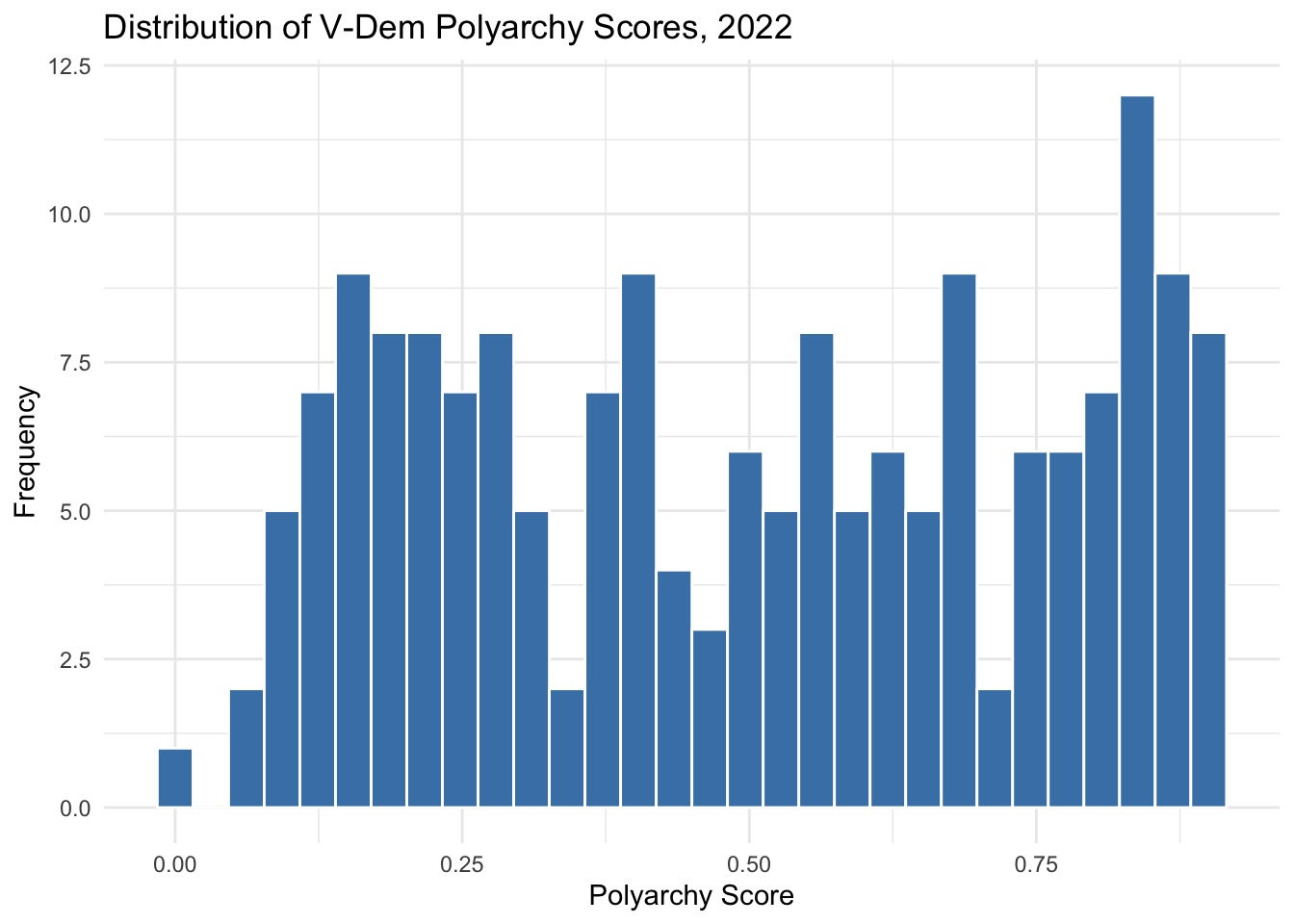
Let’s use the vdem2022 data frame that we created in the setup chunk to visualize the distribution of the V-Dem polyarchy scores for 2022:
ggplot(vdem2022, aes(x =polyarchy))+geom_histogram(bins =30, fill ="steelblue", color ="white")+theme_minimal()+labs( title ="Distribution of V-Dem Polyarchy Scores, 2022", x ="Polyarchy Score", y ="Frequency")
When we visualize polyarchy, we see that it is non-normal. The distribution appears to be multi-modal or perhaps even, with peaks occurring in multiple places. It is somewhat hard to tell what is going on with the data here.
Visualizing Distributions with Density Plots
Sometimes it can be easier to see what is happening with the distribution if we look at a density plot instead of a histogram. Density plots are similar in spirit to histograms but use a smoothed curve to estimate the shape of the distribution. Rather than count how many values fall into each bin, density plots estimate how likely it is to see values in different parts of the range.
They are particularly helpful when you want to compare distributions across groups or highlight subtler patterns that might be obscured by binning choices in a histogram. To create a density plot with ggplot2 we use the geom_density() function. This function also takes an aesthetic mapping (aes()) that specifies which variable to plot on the x-axis, and it automatically estimates the density of values across the range.
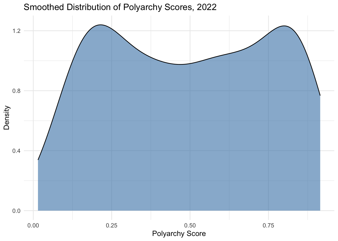
Here’s how you could create a density plot of the polyarchy score:
ggplot(vdem2022, aes(x =polyarchy))+geom_density(fill ="steelblue", alpha =0.6)+theme_minimal()+labs( title ="Smoothed Distribution of Polyarchy Scores, 2022", x ="Polyarchy Score", y ="Density")
Here it looks like we have two distinct peaks in the distribution, which suggests a that there are two groups of countries–one concentrating around a low polyarchy score and another around a high polyarchy score. In other words, the distribution appears to be bimodal, with one peak occuring at a polyarchy score of 0.2 and another around 0.8.
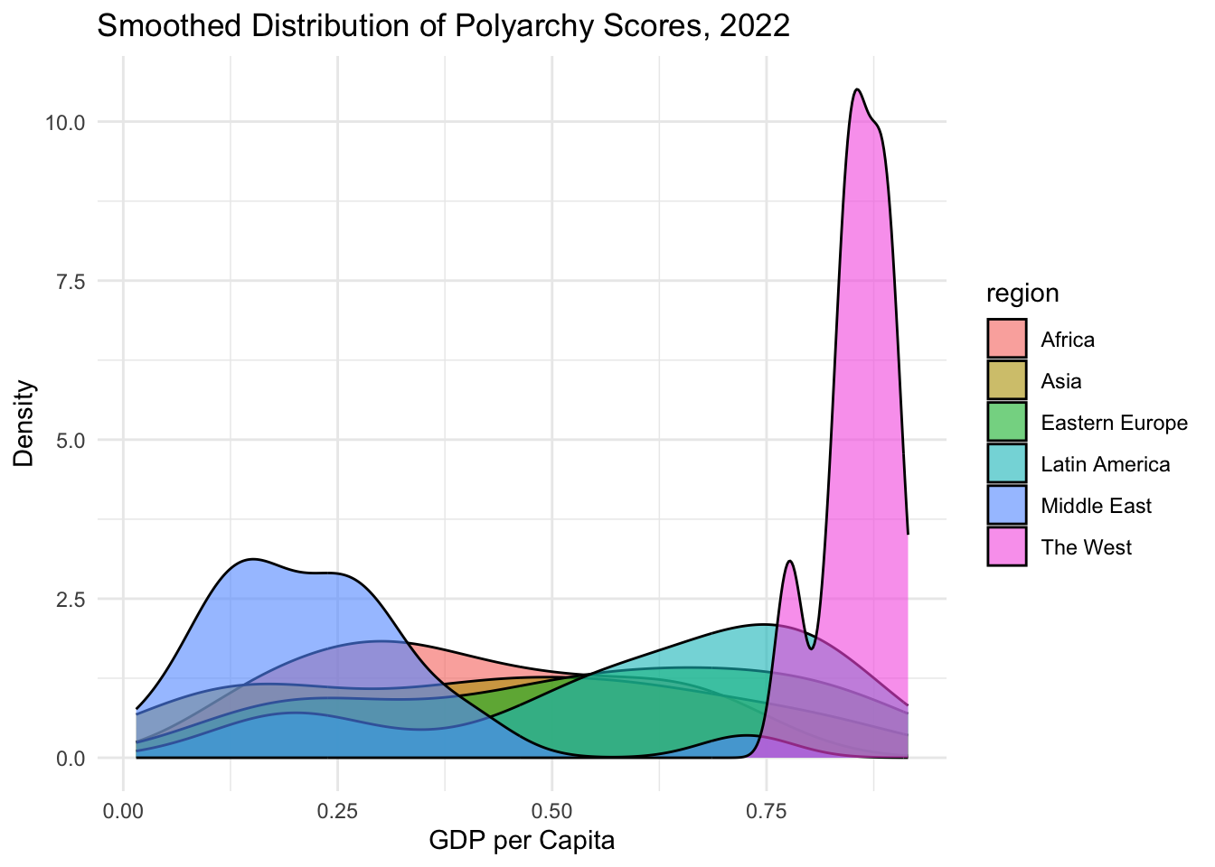
Because density plots are continuous, they’re often more elegant for comparison across groups—especially when you overlay multiple distributions on the same plot. To do that, we can add a fill aesthetic inside aes() to color the density curves by region:
ggplot(vdem2022, aes(x =polyarchy, fill =region))+geom_density(alpha =0.6)+theme_minimal()+labs( title ="Smoothed Distribution of Polyarchy Scores, 2022", x ="GDP per Capita", y ="Density")
Note
Note that if you use the fill aesthetic, you should remove the fill = argument from geom_density(). However, you should still set the alpha parameter to make the colors semi-transparent. This allows you to see overlapping areas more clearly.
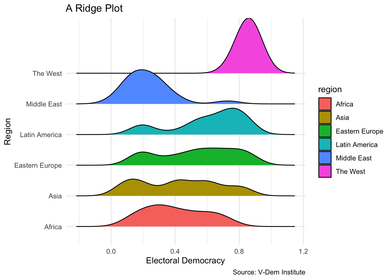
An even better solution for this is a ridge plot, which is a type of density plot that displays multiple distributions stacked on top of each other. This allows us to see how the distributions compare across groups more clearly. To create a ridge plot, we can use the geom_density_ridges() function from the ggridges package:
Now we can really see what is going on with these data. Each region has an almost unique distribution: the Middle East and Africa appear to be right-skewed; Latin America is left skewed; and the West is normally distributed. The distribution of democracy scores in other regions appears to be multimodal or unimodal. This is a very different conclusion that we would have reached had we just looked at a simple histogram!
Your Turn!!
Let’s practice visualizing a continuous variable with both histograms and density plots.
Use the vdem2022 dataset to do the following:
Create a histogram of the women_empowerment variable. Try adjusting the number of bins to see how it affects the visualization.
Now create a density plot of the women_empowerment variable. What do you notice about the shape? Does it make the distribution clearer than the histogram?
Try adding a fill = region aesthetic inside aes() to visualize the distribution of population by region. What patterns do you see? How does the distribution of women’s empowerment vary across regions?
Now try the above steps with the polarization variable. What does the distribution look like? How does it compare to the other variables?