Sampling and Uncertainty

February 7, 2025

Sampling

Sampling the act of selecting a subset of individuals, items, or data points from a larger population to estimate characteristics or metrics of the entire population
Versus a census, which involves gathering information on every individual in the population
Why would you want to use a sample?

Sampling Activity

What proportion of all milk chocolate M&Ms are blue?

M&Ms has a precise distribution of colors that it produces in its factories
M&Ms are sorted into bags in factories in a fairly random process
Each bag represents a sample from the full population of M&Ms

Activity

Get in groups of 3. Each group will have 4-5 bags of M&Ms.
Keep the contents of each bag separate, and do not eat (yet!)
Open up your first bag of M&Ms: calculate the proportion of the M&Ms that are blue. Write this down. What is your best guess (your estimate) for the proportion of all M&Ms that are blue?

Activity

Do the same as above for the rest of your bags (you should have 4-5 estimates written down)
Draw a histogram of your estimates (by hand)
Add your estimates to this Google Sheet
Add your estimates to the class histogram on the whiteboard

Let’s Analyze the Data

We will use the googlesheets4 package to pull the data into R so be sure to install it.

#install.packages("googlesheets4")

library(tidyverse)
library(googlesheets4)

gs4_deauth() # to signify no authorization required

mnm_data <- read_sheet("https://docs.google.com/spreadsheets/d/136wGKZOnwOdo3O-4bUfF_TWKBCAWQUCyiVKSY4HyYAw/edit#gid=0")

glimpse(mnm_data)

Calculate Some Summary Stats

mnm_data |>
  summarize(
    mean_blue = mean(proportion_blue),
    median_blue = median(proportion_blue),
    sd_blue = sd(proportion_blue)
  )

Now Let’s Make a Histogram

ggplot(mnm_data, aes(x = proportion_blue)) +
  geom_histogram(fill = "steelblue") +
  labs(
    title = "Percentage of Blue M&Ms",
    x = "Proportion Blue",
    y = "Count"
  )

Discuss with Neighbor

What is the histogram/distribution showing?
Based on the histogram on the board, what is your answer to the question of what proportion of all milk chocolate M&Ms are blue? Why do you give that answer?
Why do some bag of M&Ms have proportions of blues that are higher and lower than the number you gave above?
How do our estimates relate to the actual percentage of blue M&Ms manufactured (ask Google or ChatGPT)

What did we just do?

We wanted to say something about the population of M&Ms
The parameter we care about is the proportion of M&Ms that are blue
It would be impossible to conduct a census and to calculate the parameter
We took a sample from the population and calculated a sample statistic
statistical inference: act of making a guess about a population using information from a sample

What did we just do?

We completed this task many times
This produced a sampling distribution of our estimates
There is a distribution of estimates because of sampling variability
Due to random chance, one estimate from one sample can differ from another
These are foundational ideas for statistical inference that we are going to keep building on

Zooming Out

Target Population

In data analysis, we are usually interested in saying something about a Target Population.

What proportion of adult Russians support the war in Ukraine?
- Target population: adult Russians (age 18+)
How many US college students check social media during their classes?
- Target population: US college students
What percentage of M&Ms are blue?
- Target population: all of the M&Ms

Sample

In many instances, we have a Sample

We cannot talk to every Russian
We cannot talk to all college students
We cannot count all of the M&Ms

Parameters vs Statistics

The parameter is the value of a calculation for the entire target population
The statistic is what we calculate on our sample
- We calculate a statistic in order to say something about the parameter

Inference

Inference–The act of “making a guess” about some unknown
Statistical inference–Making a good guess about a population from a sample
Causal inference–Did X cause Y? [topic for later classes]

Uncertainty

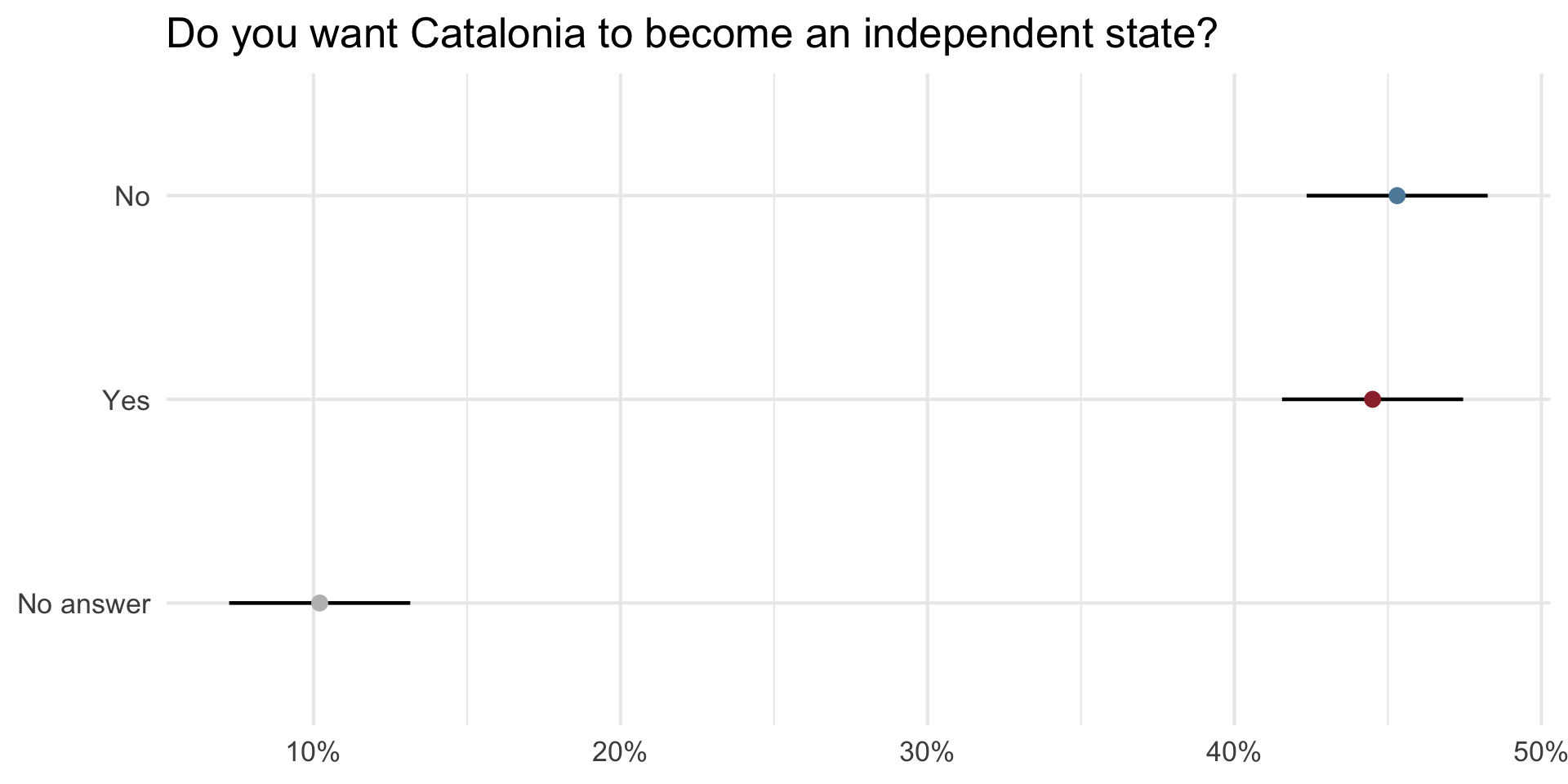
On December 19, 2014, the front page of Spanish national newspaper El País read “Catalan public opinion swings toward ‘no’ for independence, says survey”.¹

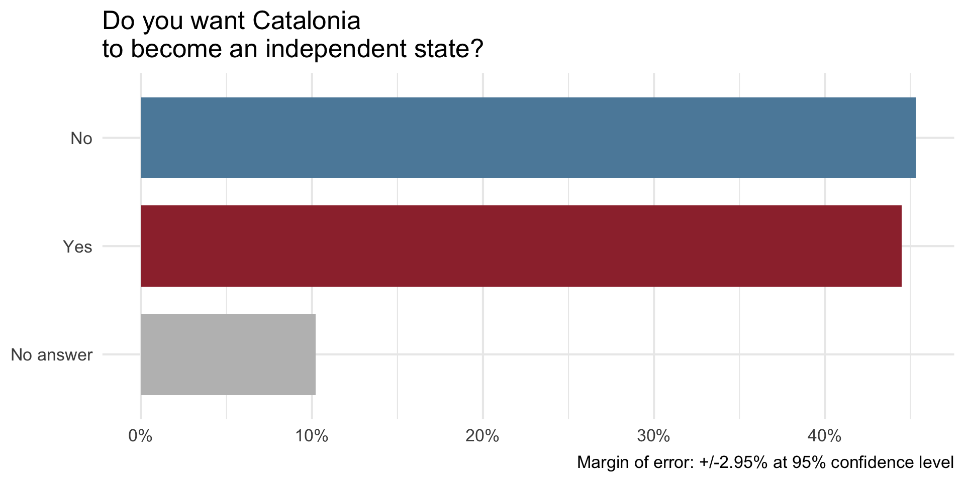
The probability of the tiny difference between the ‘No’ and ‘Yes’ being just due to random chance is very high.¹

Characterizing Uncertainty

We know from previous section that even unbiased procedures do not get the “right” answer every time
We also know that our estimates might vary from sample to sample due to random chance
Therefore we want to report on our estimate and our level of uncertainty

Characterizing Uncertainty

With M&Ms, we knew the population parameter
In real life, we do not!
We want to generate an estimate and characterize our uncertainty with a range of possible estimates

Solution: Create a Confidence Interval

A plausible range of values for the population parameter is a confidence interval.

95 percent confidence interval is standard
- We are 95% confident that the parameter value falls within the range given by the confidence interval

Ways to Estimate

Take advantage of Central Limit Theorem to estimate using math
Use simulation, bootstrapping

With Math…

\[CI = \bar{x} \pm Z \left( \frac{\sigma}{\sqrt{n}} \right)\]

\(\bar{x}\) is the sample mean,
\(Z\) is the Z-score corresponding to the desired level of confidence
\(\sigma\) is the population standard deviation, and
\(n\) is the sample size

This part here represents the standard error:

\[\left( \frac{\sigma}{\sqrt{n}} \right)\]

Standard deviation of the sampling distribution
Characterizes the spread of the sampling distribution
The bigger this is the bigger the CIs are going to be

Central Limit Theorem

\[CI = \bar{x} \pm Z \left( \frac{\sigma}{\sqrt{n}} \right)\]

This way of doing things depends on the Central Limit Theorem
As sample size gets bigger, the spread of the sampling distribution gets narrower
The shape of the sampling distributions becomes more normally distributed

\[CI = \bar{x} \pm Z \left( \frac{\sigma}{\sqrt{n}} \right)\]

This is therefore a parametric method of calculating the CI. It depends on assumptions about the normality of the distribution.

Bootstrapping

Pulling oneself up from their bootstraps …
Use the data we have to estimate the sampling distribution
We call this the bootstrap distribution
This is a nonparametric method
It does not depend on assumptions about normality

Bootstrap Process

Take a bootstrap sample - a random sample taken with replacement from the original sample, of the same size as the original sample

Calculate the bootstrap statistic - a statistic such as mean, median, proportion, slope, etc. computed on the bootstrap samples

Repeat steps (1) and (2) many times to create a bootstrap distribution - a distribution of bootstrap statistics

Calculate the bounds of the XX% confidence interval as the middle XX% of the bootstrap distribution (usually 95 percent confidence interval)

Russia

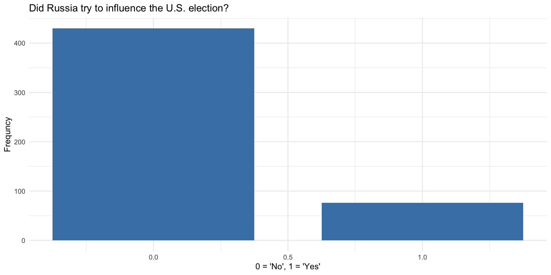
What Proportion of Russians believe their country interfered in the 2016 presidential elections in the US?

Pew Research survey
506 subjects
Data available in the openintro package

For this example, we will use data from the Open Intro package. Install that package before running this code chunk.

#install.packages("openintro")
library(openintro)

glimpse(russian_influence_on_us_election_2016)

Rows: 506
Columns: 1
$ influence_2016 <chr> "Did not try", "Did not try", "Did not try", "Don't kno…

Let’s use mutate() to recode the qualitative variable as a numeric one…

russiaData <- russian_influence_on_us_election_2016 |> 
  mutate(try_influence = ifelse(influence_2016 == "Did try", 1, 0))

Now let’s calculate the mean and standard deviation of the try_influence variable…

russiaData |>
  summarize( 
          mean = mean(try_influence),
          sd = sd(try_influence)
  )

# A tibble: 1 × 2
   mean    sd
  <dbl> <dbl>
1 0.150 0.358

And finally let’s draw a bar plot…

ggplot(russiaData, aes(x = try_influence)) +
  geom_bar(fill = "steelblue", width = .75) +
  labs(
    title = "Did Russia try to influence the U.S. election?",
    x = "0 = 'No', 1 = 'Yes'",
    y = "Frequncy"
  ) +
  theme_minimal()

Bootstrap with `tidymodels`

Install tidymodels before running this code chunk…

#install.packages("tidymodels")
library(tidymodels)

set.seed(66)
boot_dist <- russiaData |>
  # specify the variable of interest
  specify(response = try_influence) |>
  # generate 10000 bootstrap samples
  generate(reps = 10000, type = "bootstrap") |>
  # calculate the mean of each bootstrap sample
  calculate(stat = "mean")

glimpse(boot_dist)

Rows: 10,000
Columns: 2
$ replicate <int> 1, 2, 3, 4, 5, 6, 7, 8, 9, 10, 11, 12, 13, 14, 15, 16, 17, 1…
$ stat      <dbl> 0.1146245, 0.1442688, 0.1343874, 0.1877470, 0.1521739, 0.138…

Calculate the mean of the bootstrap distribution (of the means of the individual draws)…

boot_dist |> summarize(mean = mean(stat))

# A tibble: 1 × 1
   mean
  <dbl>
1 0.150

Calculate the confidence interval. A 95% confidence interval is bounded by the middle 95% of the bootstrap distribution.

boot_dist |>
  summarize(lower = quantile(stat, 0.025),
            upper = quantile(stat, 0.975))

# A tibble: 1 × 2
  lower upper
  <dbl> <dbl>
1 0.119 0.182

Create upper and lower bounds for visualization.

# for using these values later
lower_bound <- boot_dist |> summarize(lower_bound = quantile(stat, 0.025)) |> pull() 
upper_bound <- boot_dist |> summarize(upper_bound = quantile(stat, 0.975)) |> pull()

Visualize with a histogram

ggplot(data = boot_dist, mapping = aes(x = stat)) +
  geom_histogram(binwidth =.01, fill = "steelblue4") +
  geom_vline(xintercept = c(lower_bound, upper_bound), color = "darkgrey", size = 1, linetype = "dashed") +
  labs(title = "Bootstrap distribution of means",
       subtitle = "and 95% confidence interval",
       x = "Estimate",
       y = "Frequency") +
  theme_bw()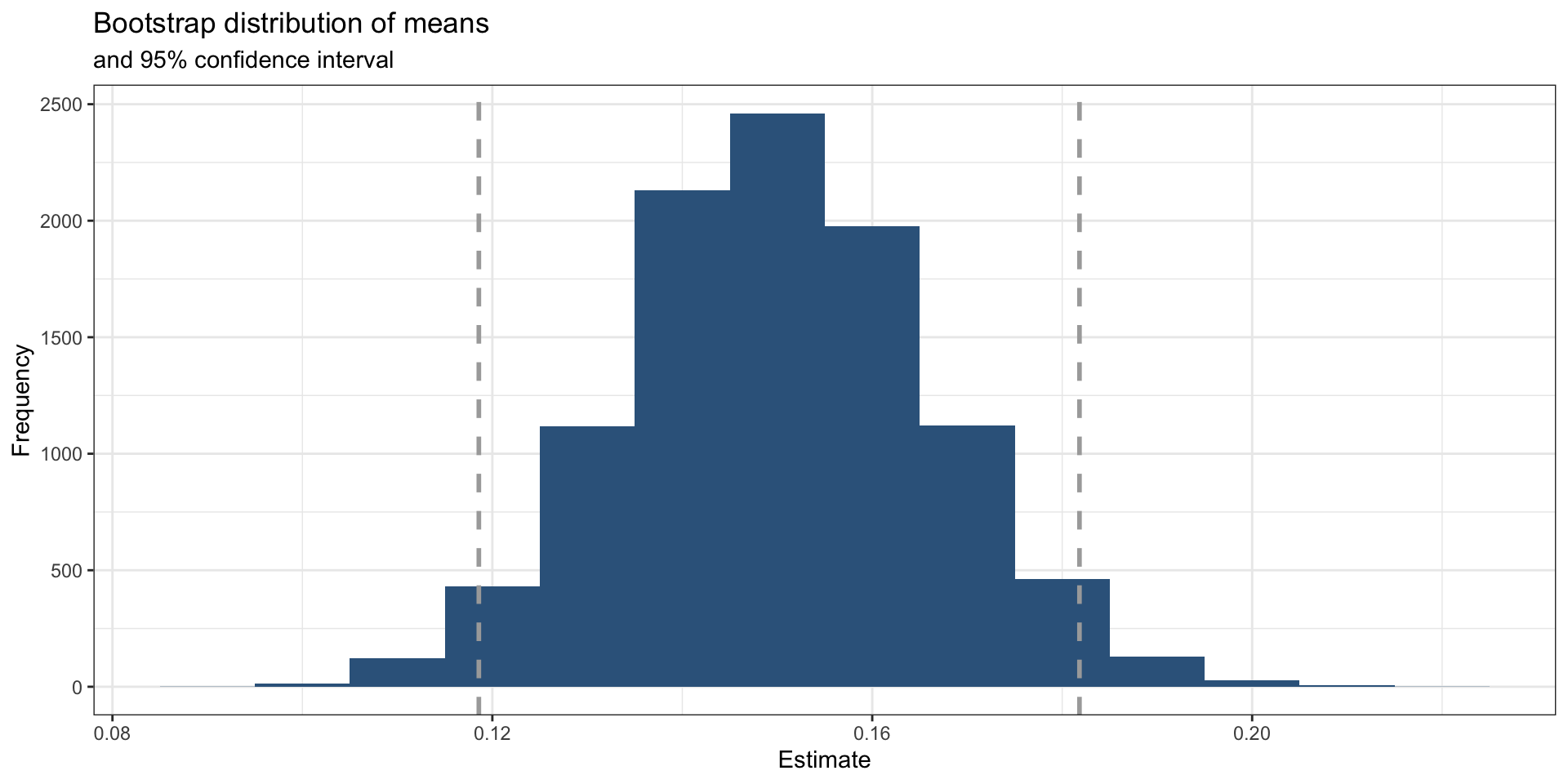

Or use the `infer` package

ci <- boot_dist |> get_ci(level = 0.95) 

ci

# A tibble: 1 × 2
  lower_ci upper_ci
     <dbl>    <dbl>
1    0.119    0.182

Or use the `infer` package

boot_dist |>
  visualize() +
  shade_ci(ci, color = "red", fill = NULL) +
  labs( 
    title = "Distribution of the Means of the Bootstrap Samples",
    x = "Mean",
    y = "Count"
  ) +
  theme_minimal()

Or use the `infer` package

boot_dist |>
  visualize() +
  shade_ci(ci, color = "red", fill = NULL) +
  labs( 
    title = "Distribution of the Means of the Bootstrap Samples",
    x = "Mean",
    y = "Count"
  ) +
  theme_minimal()

Interpret the confidence interval

The 95% confidence interval was calculated as (lower_bound, upper_bound). Which of the following is the correct interpretation of this interval?

(a) 95% of the time the percentage of Russian who believe that Russia interfered in the 2016 US elections is between lower_bound and upper_bound.

(b) 95% of all Russians believe that the chance Russia interfered in the 2016 US elections is between lower_bound and upper_bound.

(c) We are 95% confident that the proportion of Russians who believe that Russia interfered in the 2016 US election is between lower_bound and upper_bound.

(d) We are 95% confident that the proportion of Russians who supported interfering in the 2016 US elections is between lower_bound and upper_bound.

Your Turn!

Change the reps argument in the generate() function to something way smaller, like 100. What happens to your estimates?
Try progressively higher numbers. What happens to your estimates as the number of reps increases?

Why did we do these simulations?

They provide a foundation for statistical inference and for characterizing uncertainty in our estimates
The best research designs will try to maximize or achieve good balance on bias vs precision

Sampling and Uncertainty

Sampling

Sampling Activity

What proportion of all milk chocolate M&Ms are blue?

Activity

Activity

Let’s Analyze the Data

Calculate Some Summary Stats

Now Let’s Make a Histogram

Discuss with Neighbor

What did we just do?

What did we just do?

Zooming Out

Target Population

Sample

Parameters vs Statistics

Inference

Uncertainty

Characterizing Uncertainty

Characterizing Uncertainty

Solution: Create a Confidence Interval

Ways to Estimate

With Math…

Central Limit Theorem

Bootstrapping

Bootstrap Process

Russia

Bootstrap with tidymodels

Or use the infer package

Or use the infer package

Or use the infer package

Interpret the confidence interval

Your Turn!

Why did we do these simulations?

Bootstrap with `tidymodels`

Or use the `infer` package

Or use the `infer` package

Or use the `infer` package