Hypothesis Testing 2

Reletionship Between Two Variables

February 7, 2025

Hypotheses

• Null hypothesis: there is no relationship between treatment and outcome, the difference is due to chance
• Alternative hypothesis: there is a relationship, the difference is not due to chance

Approach

• Under the null hypothesis, treatment has NO impact on y (the outcome)
• This means that if we were to change the values of the treatment variable, the values on y would stay the same

Approach

• So…we can simulate the null distribution by:
  • Reshuffling the treatment variable
  • Calculating the treatment effect
  • Repeating many times

• Then we can ask: how likely would we be to observe the treatment effect in our data, if there is no effect of the treatment?

Résumé Experiment Example

Bertrand and Mullainathan studied racial discrimination in responses to job applications in Chicago and Boston. They sent 4,870 résumés, randomly assigning names associated with different racial groups. - Data are in openintro package as an object called resume - I will save as myDat

library(openintro)
myDat <- resume 

Callbacks by Race

Remember, race of applicant is randomly assigned.

library(tidyverse)

mns <- myDat |>
  group_by(race) |> 
  summarize(calls = mean(received_callback))
mns

# A tibble: 2 × 2
  race   calls
  <chr>  <dbl>
1 black 0.0645
2 white 0.0965

Let’s save the means for white and black applicants.

mean_white = mns$calls[2]
mean_black = mns$calls[1]

And calculate the treatment effect. The treatment effect is the difference in means.

teffect <- mean_white - mean_black
teffect

[1] 0.03203285

Before formal tests, let’s look at the data–the estimates and the confidence intervals…

First, let’s make the CIs for the white applicants.

library(tidymodels)
boot_df_white <- myDat |>
  filter(race == "white") |> 
  specify(response = received_callback) |>  
  generate(reps = 15000, type = "bootstrap") |> 
  calculate(stat = "mean")
lower_bound_white <- boot_df_white |> summarize(lower_bound_white = quantile(stat, 0.025)) |> pull() 
upper_bound_white <- boot_df_white |> summarize(upper_bound_white = quantile(stat, 0.975)) |> pull() 

Now, let’s create the CIs for black applicants.

boot_df_black <- myDat |>
  filter(race == "black") |> 
  specify(response = received_callback) |>  
  generate(reps = 15000, type = "bootstrap") |> 
  calculate(stat = "mean")
lower_bound_black <- boot_df_black |> summarize(lower_bound_black = quantile(stat, 0.025)) |> pull() 
upper_bound_black <- boot_df_black |> summarize(upper_bound_black = quantile(stat, 0.975)) |> pull() 

Now, let’s tidy the data for plotting.

plotData <- tibble(
  race = c("Black", "White"),
  meanCalls = c(mean_black, mean_white),
  lower95 = c(lower_bound_black, lower_bound_white),
  upper95 = c(upper_bound_black, upper_bound_white)
)
plotData

# A tibble: 2 × 4
  race  meanCalls lower95 upper95
  <chr>     <dbl>   <dbl>   <dbl>
1 Black    0.0645  0.0550  0.0743
2 White    0.0965  0.0846  0.108 

Plot

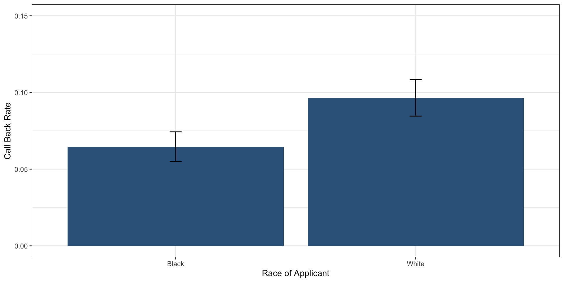
Plot

ggplot(plotData, aes(y = meanCalls, x = race, ymin = lower95, ymax = upper95)) +
  geom_col(fill = "steelblue4") +
  geom_errorbar(width = .05) +
  theme_bw()  +
  ylim(0, .15) +
  labs(x = "Race of Applicant",
       y = "Call Back Rate")

Is this evidence of racial discrimination?

• What is the null hypothesis?

• What is the alternative hypothesis?

• How can we formally test the null hypothesis to decide whether to reject it?

Formal Hypothesis Test

• Calculate the difference in means (White - Black)
• Shuffle the race variable
• Calculate the difference in means for the shuffled data
• Repeat many times
• Simulates the null distribution of differences in callbacks

Hypothetical Original Data

Applicant	Race	Callback
A	Black	Yes
B	Black	No
C	Black	No
D	White	Yes
E	White	No
F	White	No

Step 1: Calculate Original Difference in Callback Rates

• Objective: Understand initial association between race and callback rates

Step 2: Shuffle (Permute) the Race Variable

• Method: Randomly reassign race labels, keeping callback outcomes fixed

Hypothetical Shuffled Data

Applicant	Race (Shuffled)	Callback
A	White	Yes
B	Black	No
C	White	No
D	White	Yes
E	Black	No
F	Black	No

Step 3: Calculate Difference in Callback Rates Again

• After Shuffling: Calculate the difference in callback rates between Black and White groups
• Purpose: Determine if observed difference is due to chance

Repeat Many Times

• Repeat shuffling 5000 times to generate a distribution of differences by chance
• Test: Compare observed difference to null distribution to assess effect of race on callbacks
• If observed difference is extreme (p-value is low), reject the null hypothesis

Simulating with tidymodels

In real life we are going to use the tidymodels package to do the simulation for us.

null_dist <- myDat |>
  specify(response = received_callback, explanatory = race) |>
  hypothesize(null = "independence") |>
  generate(5000, type = "permute") |>
  calculate(stat = "diff in means", 
            order = c("white", "black")) # 

Get the p-value

Let’s get the p-value with get_pvalue from the infer package.

get_p_value(null_dist, obs_stat = teffect, direction = "greater")

# A tibble: 1 × 1
  p_value
    <dbl>
1       0

Visualize the Null Distribution

visualize(null_dist) +
  shade_p_value(obs_stat = teffect, direction = "greater") +
  labs(
    x = "Estimated Difference under the Null",
    y = "Count"
  ) + 
  theme_bw()

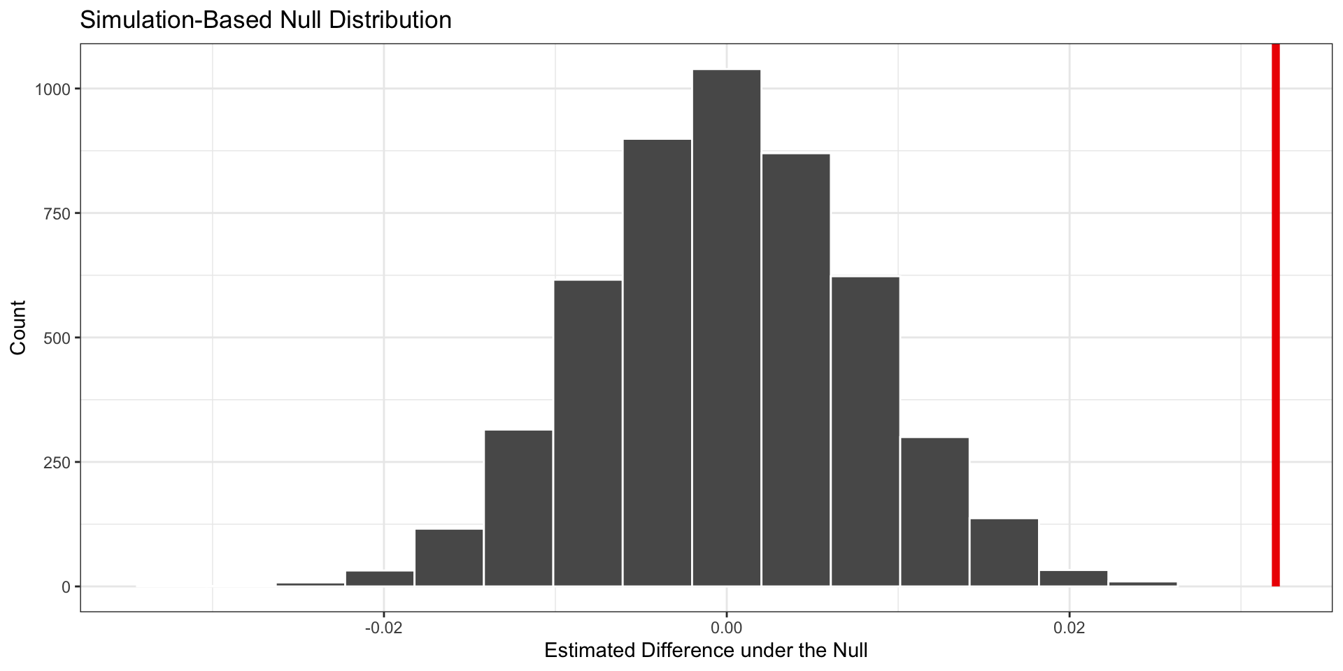
What should we conclude?

• The p-value is very small (below .05 threshold)
• Therefore, we reject the null hypothesis: the racial gap is extremely unlikely to have occurred due to chance alone
• This is evidence of racial discrimination

Your Turn!

• Use the gender variable in the resume data to assess whether there is gender discrimination in call backs
• Plot means and 95% confidence intervals for the call back rate for men and women
• Write the null and alternative hypotheses
• Simulate the null distribution
• Visualize the null distribution and the gender gap
• Calculate the p-value
• What do you conclude from your test?