Linear Regression

October 16, 2024

Modeling

Use models to explore the relationship between variables and to make predictions
Explaining relationships (usually interested in causal relationships, but not always)
- Does oil wealth impact regime type?
Predictive modeling
- Where is violence most likely to happen in (country X) during their next election?
- Is this email spam?

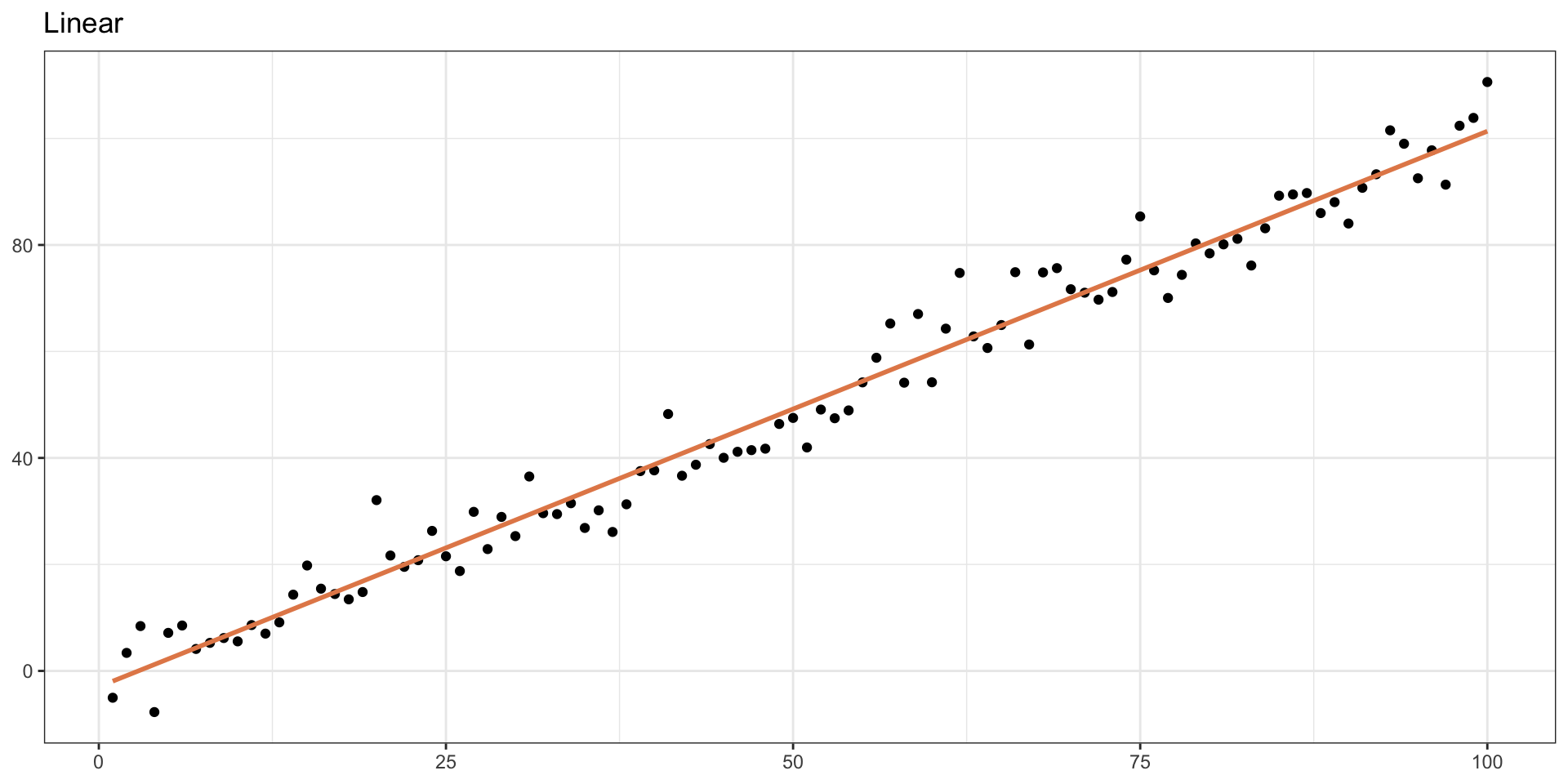
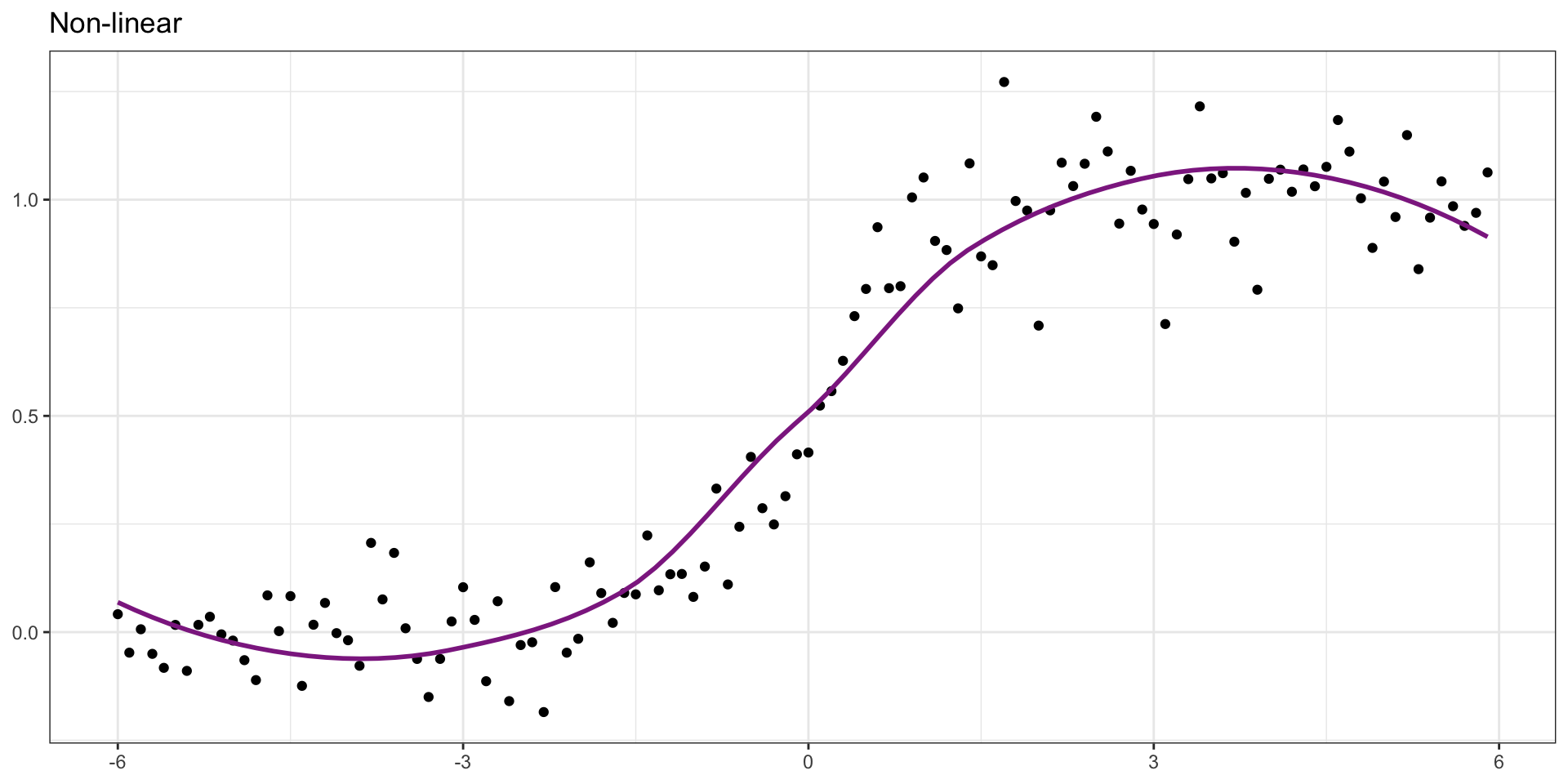
Modeling

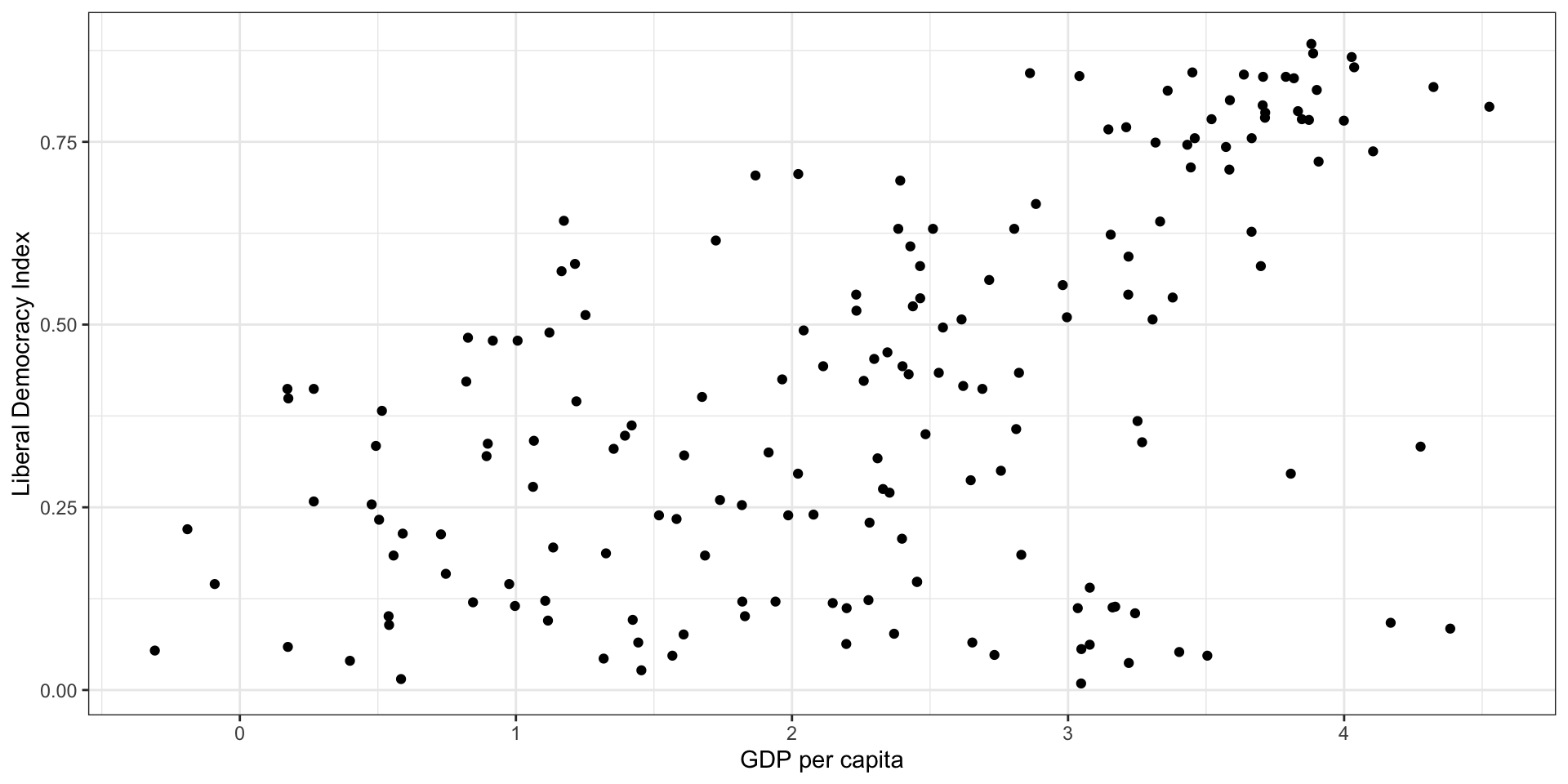
Example: GDP per capita and Democracy

Pull in the VDEM Data

library(vdemlite)

model_data <- fetchdem(indicators = c("v2x_libdem", "e_gdppc"),
                       start_year = 2019, end_year = 2019) |>
  rename(
    country = country_name, 
    lib_dem = v2x_libdem, 
    wealth = e_gdppc
    ) 

glimpse(model_data)

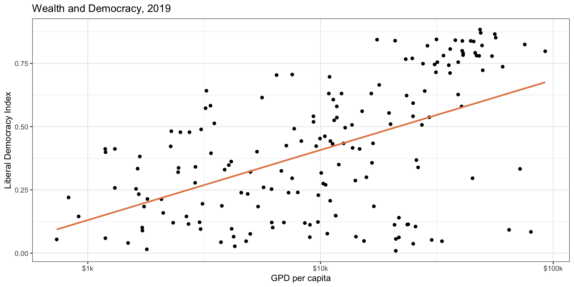
Plot the Data

ggplot(model_data, aes(x = wealth, y = lib_dem)) +
  geom_point() +
  geom_smooth(method = "lm", color = "#E48957", se = FALSE) +
  scale_x_log10(label = scales::label_dollar(suffix = "k")) +
  labs(
    title = "Wealth and Democracy, 2019",
    x = "GPD per capita", 
    y = "Liberal Democracy Index") +
  theme_bw()

Models as Functions

We can represent relationships between variables using functions
A function is a mathematical concept: the relationship between an output and one or more inputs
- Plug in the inputs and receive back the output
Example: The formula $y = 3x + 7$ is a function with input $x$ and output $y$.
- If $x$ is $5$, $y$ is $22$,
- $y = 3 \times 5 + 7 = 22$

Quant Lingo

Response variable: Variable whose behavior or variation you are trying to understand, on the y-axis in the plot
- Dependent variable
- Outcome variable
- Y variable
Explanatory variables: Other variables that you want to use to explain the variation in the response, on the x-axis in the plot
- Independent variables
- Predictors

Linear model with one explanatory variable…

$Y = a + bX$
$Y$ is the outcome variable
$X$ is the explanatory variable
$a$ is the intercept: the predicted value of $Y$ when $X$ is equal to 0
$b$ is the slope of the line (rise over run)

Quant Lingo

Predicted value: Output of the model function
- The model function gives the typical (expected) value of the response variable conditioning on the explanatory variables
- We often call this $\hat{Y}$ to differentiate the predicted value from an observed value of Y in the data
Residuals: A measure of how far each case is from its predicted value (based on a particular model)
- Residual = Observed value ($Y$) - Predicted value ($\hat{Y}$)
- How far above/below the expected value each case is

Caution

Note that for the next few examples we will be analyzing GDP per capita on a log scale.

Residuals

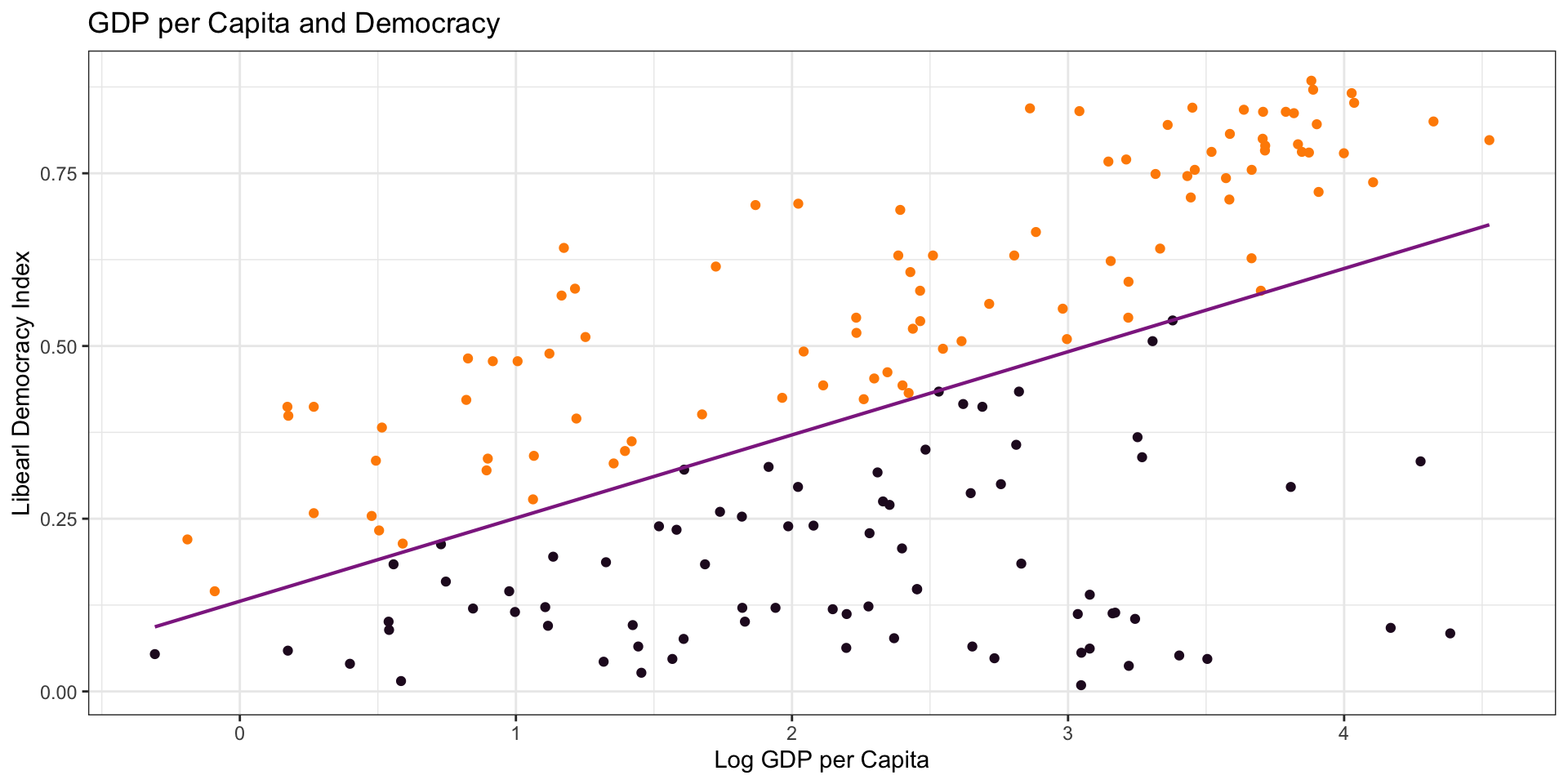
Linear Model

$\hat{Y} = a + b \times X$

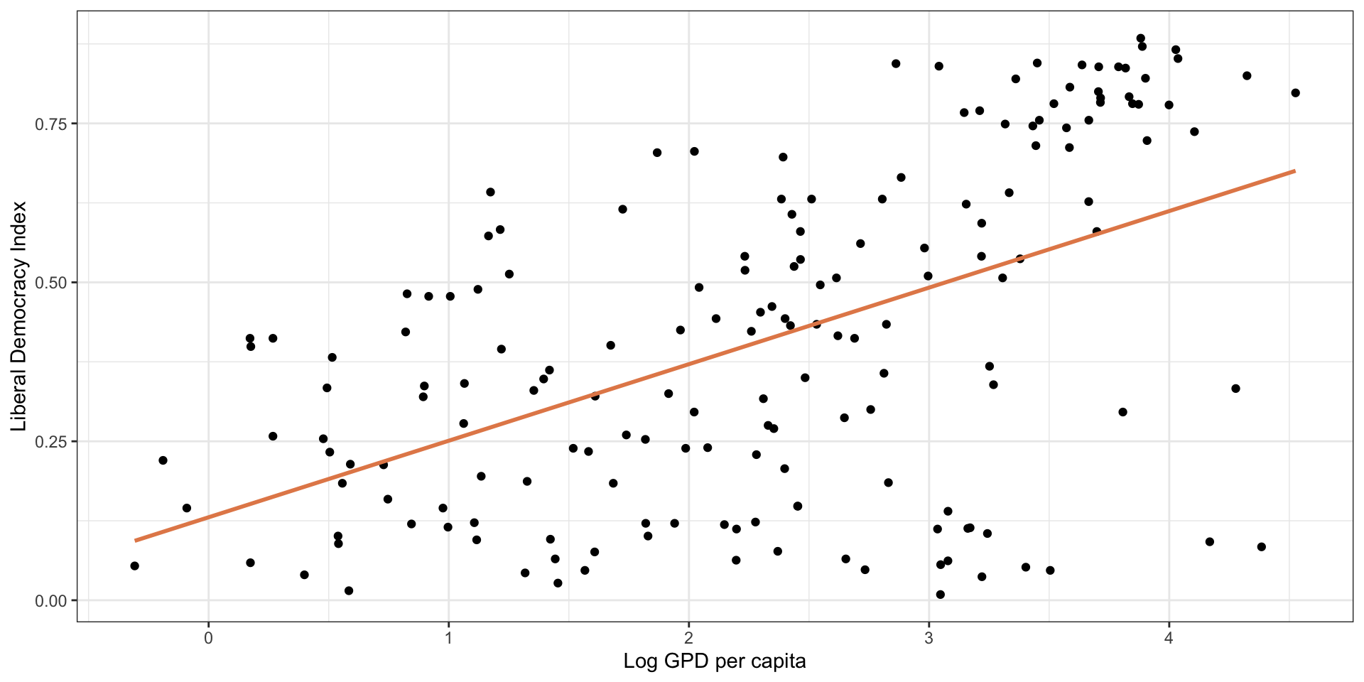
$\hat{Y} = 0.13 + 0.12 \times X$

Linear Model: Interpretation

$\hat{Y} = a + b \times X$
$\hat{Y} = 0.13 + 0.12 \times X$

What is the interpretation of our estimate of $a$?

$\hat{Y} = 0.13 + 0.12 \times 0$
$\hat{Y} = 0.13$

$a$ is our predicted level of democracy when GDP per capita is 0.

Linear Model: Interpretation

$\hat{Y} = a + b \times X$
$\hat{Y} = 0.13 + 0.12 \times X$

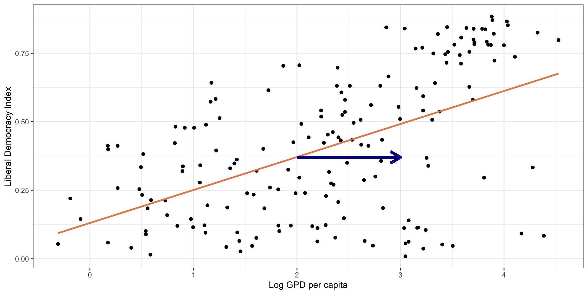
What is interpretation of our estimate of $b$?

$\hat{Y} = a + \frac{Rise}{Run} \times X$
$\hat{Y} = a + \frac{Change Y}{Change X} \times X$

Linear Model: Interpretation

$b = \frac{Change Y}{Change X}$
$0.12 = \frac{Change Y}{Change X}$
${Change Y} = 0.12 * {ChangeX}$

When $ChangeX = 1$:
${Change Y = 0.12}$

$b$ is the predicted change in $Y$ associated with a ONE unit change in X.

Linear Model: Interpretation

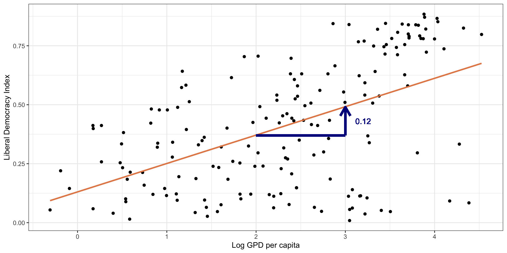
Interpreting the Coefficient for log(Wealth)

Model: Democracy = 0.12 × log(Wealth)
Coefficient Interpretation:
- A 1% increase in GDP per capita is associated with a 0.0012 increase in the democracy score
- Doubling GDP per capita (e.g., from $10,000 to $20,000) increases the democracy score by 0.12 points
In Dollar Terms:
- If GDP per capita increases by 10% (e.g., from $10,000 to $11,000), the democracy score is expected to increase by 0.012 points

Linear Model: Interpretation

Is this the causal effect of GDP per capita on liberal democracy?

No! It is only the association…

To identify causality we need other methods (beyond the scope of this course).

Your Task

An economist is interested in the relationship between years of education and hourly wages. They estimate a linear model with estimates of $a$ and $b$ as follows:

$\hat{Y} = 9 + 1.60*{YrsEdu}$

1. Interpret $a$ and $b$
2. What is the predicted hourly wage for those with 10 years of education?
3. How about for those with a high school diploma? (12 yrs)
4. What about a college degree? (16 yrs)

Next step

Linear model with one predictor: $Y = a + bX$
For any given data…
How do we figure out what the best values are for $a$ and $b$??

Estimation

Linear Model with Single Predictor

Goal: Estimate Democracy score ($\hat{Y_{i}}$) of a country given level of GDP per capita ($X_{i}$).

Or: Estimate relationship between GDP per capita and democracy.

Linear Model with Single Predictor

Estimate Model

model1 <-  lm(lib_dem ~ log_wealth, data = modelData) 

summary(model1)


Call:
lm(formula = lib_dem ~ log_wealth, data = modelData)

Residuals:
     Min       1Q   Median       3Q      Max 
-0.57441 -0.14334  0.03911  0.18730  0.37017 

Coefficients:
            Estimate Std. Error t value Pr(>|t|)    
(Intercept)  0.13051    0.03806   3.429 0.000758 ***
log_wealth   0.12040    0.01471   8.188 5.75e-14 ***
---
Signif. codes:  0 '***' 0.001 '**' 0.01 '*' 0.05 '.' 0.1 ' ' 1

Residual standard error: 0.2233 on 172 degrees of freedom
  (5 observations deleted due to missingness)
Multiple R-squared:  0.2805,    Adjusted R-squared:  0.2763 
F-statistic: 67.04 on 1 and 172 DF,  p-value: 5.754e-14

In equation form… How do we interpret the model?

\[\widehat{Democracy}_{i} = 0.13 + 0.12 * {loggdppc}_{i}\]

Question

How do we get the “best” values for the slope and intercept?

How would you draw the “best” line?

Least squares regression

Remember the residual is the difference between the actual value and the predicted value

The regression line minimizes the sum of squared residuals.

Least squares regression

Residual for each point is: $e_i = y_i - \hat{y}_i$
Least squares regression line minimizes $\sum_{i = 1}^n e_i^2$.

Why do we square the residual?

Why not take absolute value?
- Principle: larger penalty for residuals further away
- Math: makes the math easier and some nice properties (not our concern here…)

Least squares regression

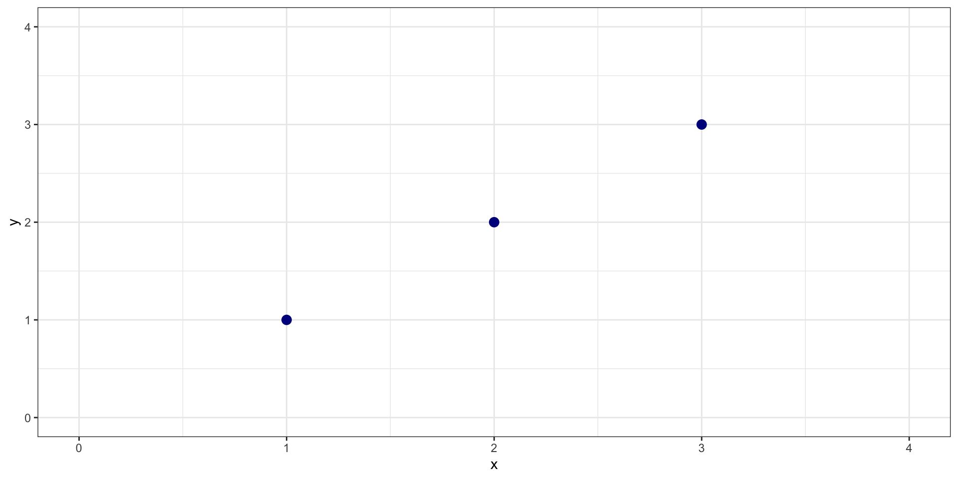
Very Simple Example

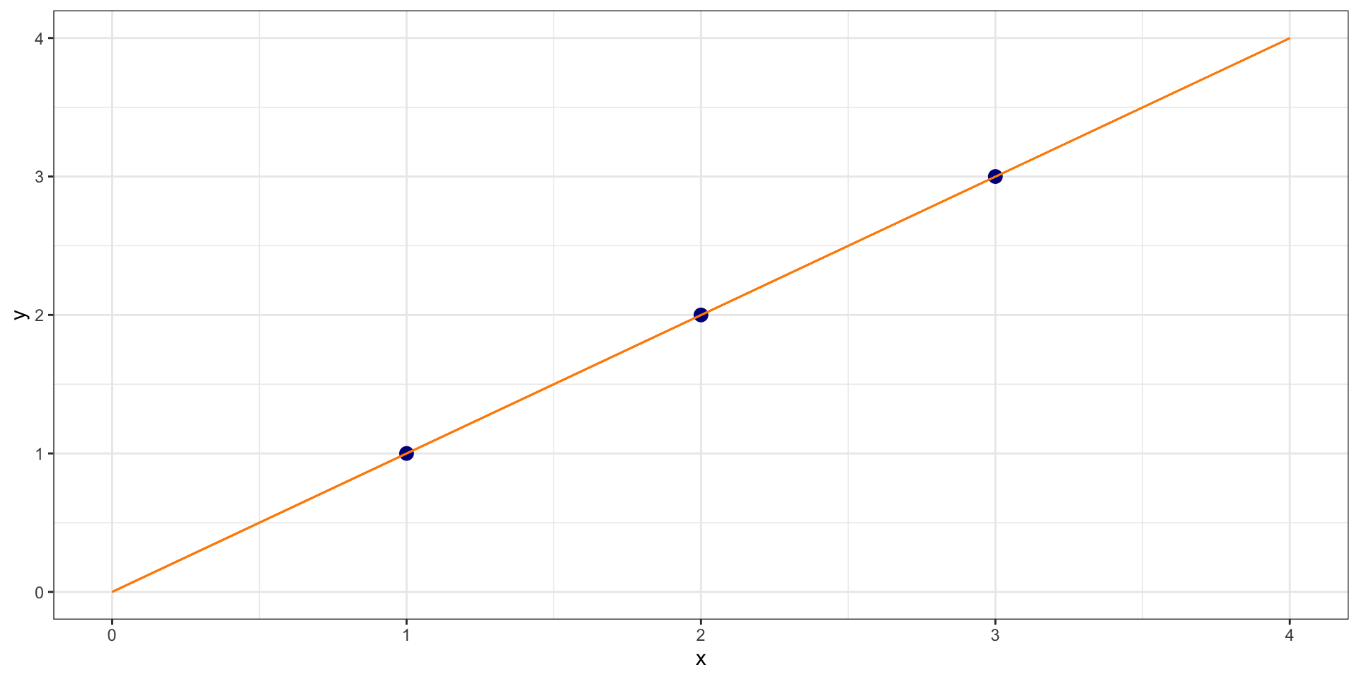
What should the slope and intercept be?

Example

$\hat{Y} = 0 + 1*X$

Example

What is the sum of squared residuals?

Example

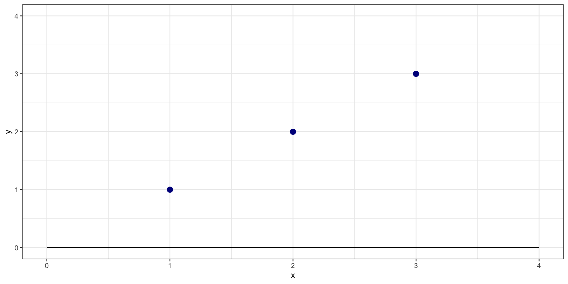
What is sum of squared residuals for $y = 0 + 0*X$?

Example

What is sum of squared residuals for $y = 0 + 0*X$?

(1-0)^2 + (2-0)^2 + (3-0)^2

[1] 14

Example

What is sum of squared residuals for $y = 0 + 2*X$?

Example

What is sum of squared residuals for $y = 0 + 2*X$?

(1-2)^2 + (2-4)^2 + (3-6)^2

[1] 14

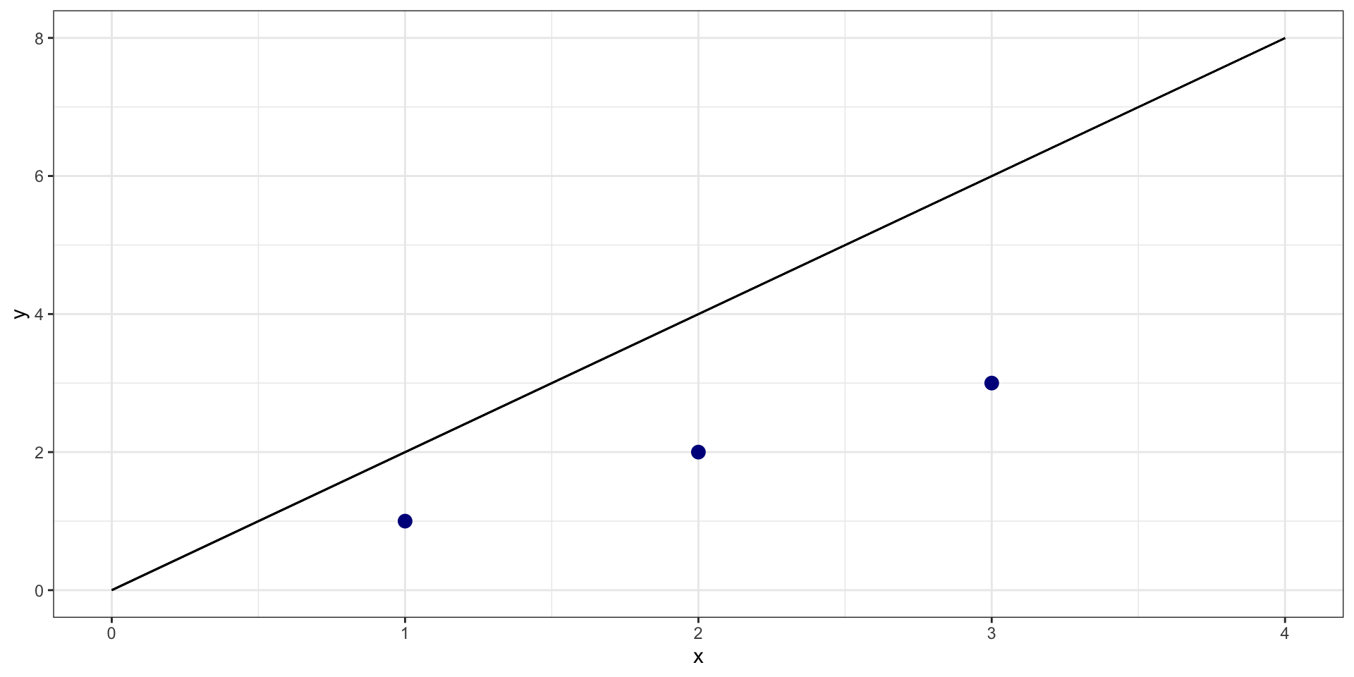
One more…

What is sum of squared residuals for $y = 0 + -1*X$?

One more…

What is sum of squared residuals for $y = 0 + -1*X$?

(1+1)^2 + (2+2)^2 + (3+3)^2

[1] 56

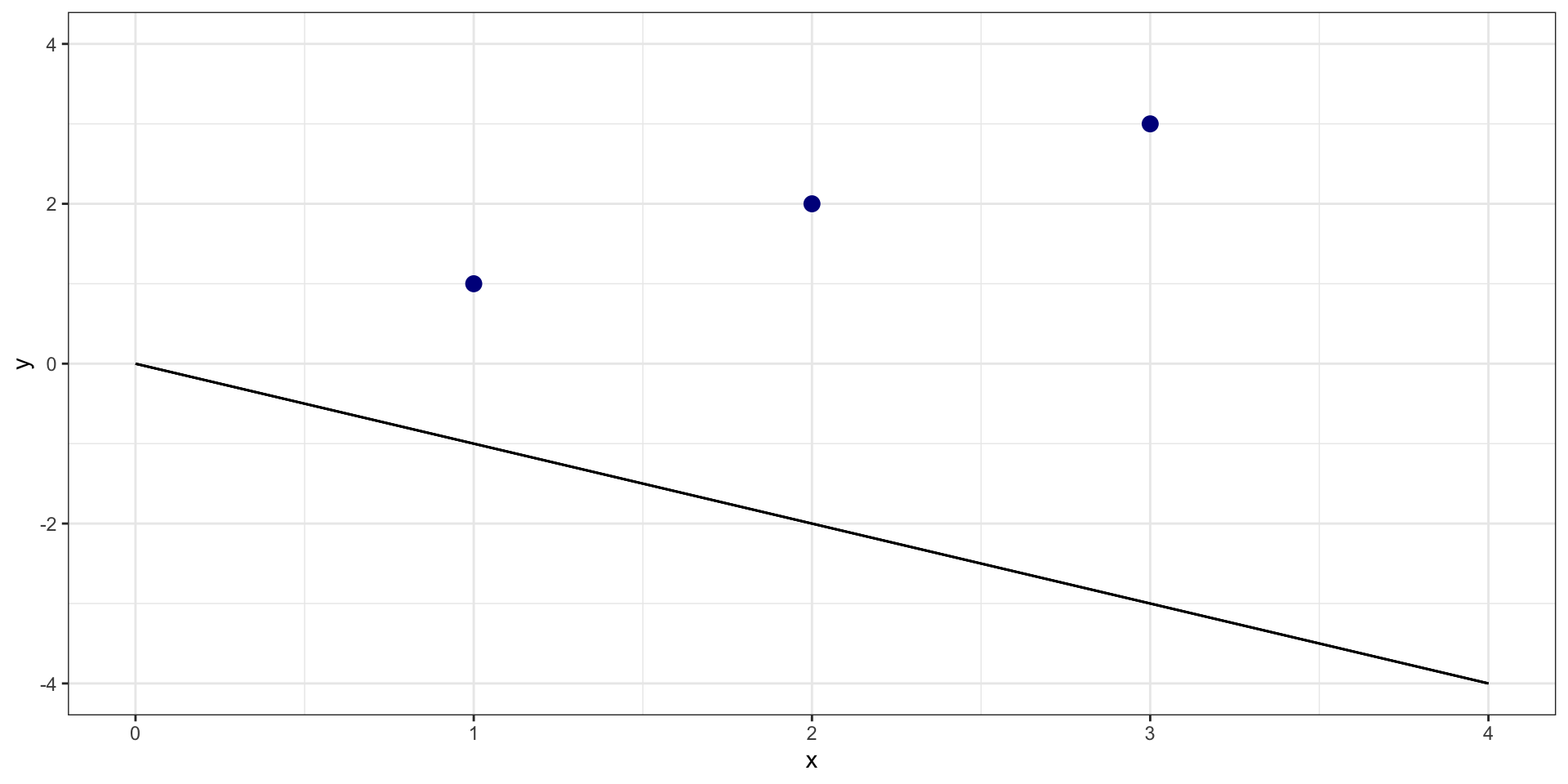
Cost Function

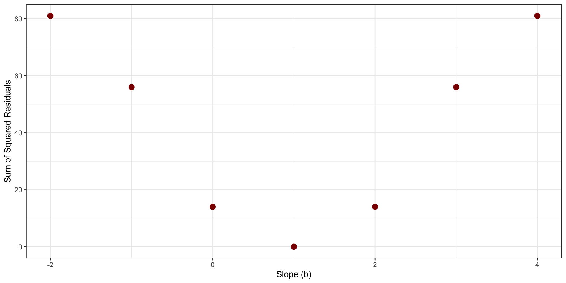
Sum of Squared Residuals as function of possible values of $b$

Least Squares Regression

When we estimate a least squares regression, it is looking for the line that minimizes sum of squared residuals
In the simple example, I set $a=0$ to make it easier. More complicated when searching for combination of $a$ and $b$ that minimize, but same basic idea

Least Squares Regression

There is a way to solve for this analytically for linear regression (i.e., by doing math…)

– They made us do this in grad school…

In machine learning, people also use gradient descent algorithm in which the computer searches over possible combinations of $a$ and $b$ until it settles on the lowest point.